Summary

One page for the numbers and the caveats. Everything here is measured on the machine in methodology — NVIDIA RTX A2000 Laptop GPU (4 GB, driver 560.35.03 / CUDA 12.6), Intel Core i7-11850H, Python 3.10.12, CuPy 14.2.0, NumPy 2.2.6, pymapf 0.8.0, on 2026-08-20 — with three seeds per cell and the raw rows committed under benchmarks/experiments/. A number without conditions is not a result, so every row below carries its own.

Headline

Workload	conditions	pymapf	cuplan CPU	cuplan CUDA
Prioritized planning	64² grid, 5% obstacles, 128 agents, 3 seeds	47.95 s	0.590 s	0.289 s ¹
Prioritized planning	64² grid, 5% obstacles, 256 agents, 3 seeds	timeout at 60 s	1.19 s	— ²
PIBT	64² grid, 5% obstacles, 512 agents, 3 seeds	5.35 s	0.541 s	— ²
Batched BFS	256² grid, 15% obstacles, 1024 distance maps, 3 seeds	n/a ³	62.09 s	1.87 s
Flocking (Boids)	2048 agents, 200 steps, 3 seeds	n/a ⁴	92.16 s	0.377 s
Velocity obstacles	512 agents, 80 steps, 3 seeds	n/a ⁴	31.21 s	5.57 s

Medians over seeds {0, 1, 2}; wall time for the whole solve() / run() call, host/device transfers included. ¹ 2 of 3 seeds — the third is where the device fault started. ² CUDA rows lost to the device fault; see what is missing. ³ pymapf has no batched distance-map primitive; its per-agent Dijkstra cost is inside the solver rows above. ⁴ pymapf's simulators update agents sequentially within a timestep, so a wall-clock comparison would time a different problem — see the semantics note.

Three claims fall out of that table, with the conditions attached:

• Most of the win against pymapf is not the GPU. Prioritized planning on a 64² grid at 5% density with 128 agents is 78.5× faster on cuplan's CPU backend, and the device adds a further 2.0× on top. The batched-BFS oracle and the dense reservation table do that work; NumPy is enough to get it.
• The GPU pays through batch size, and the exchange rate varies by two orders of magnitude. 245× for flocking at 2048 agents; 33× for 1024 distance maps on a 256² grid; 5.6× for 512 velocity-obstacle agents; 2.0× for prioritized planning. The difference is how much of the workload is a single wide kernel and how much is a sequential loop the host must drive.
• No speedup was bought with a worse plan. On all 105 MAPF instances solved by both cuplan backends, the CPU and CUDA solutions have identical sum of costs and identical makespan. Against pymapf on 197 shared instances the median sum-of-costs ratio is exactly 1.0000.

Where the crossovers are

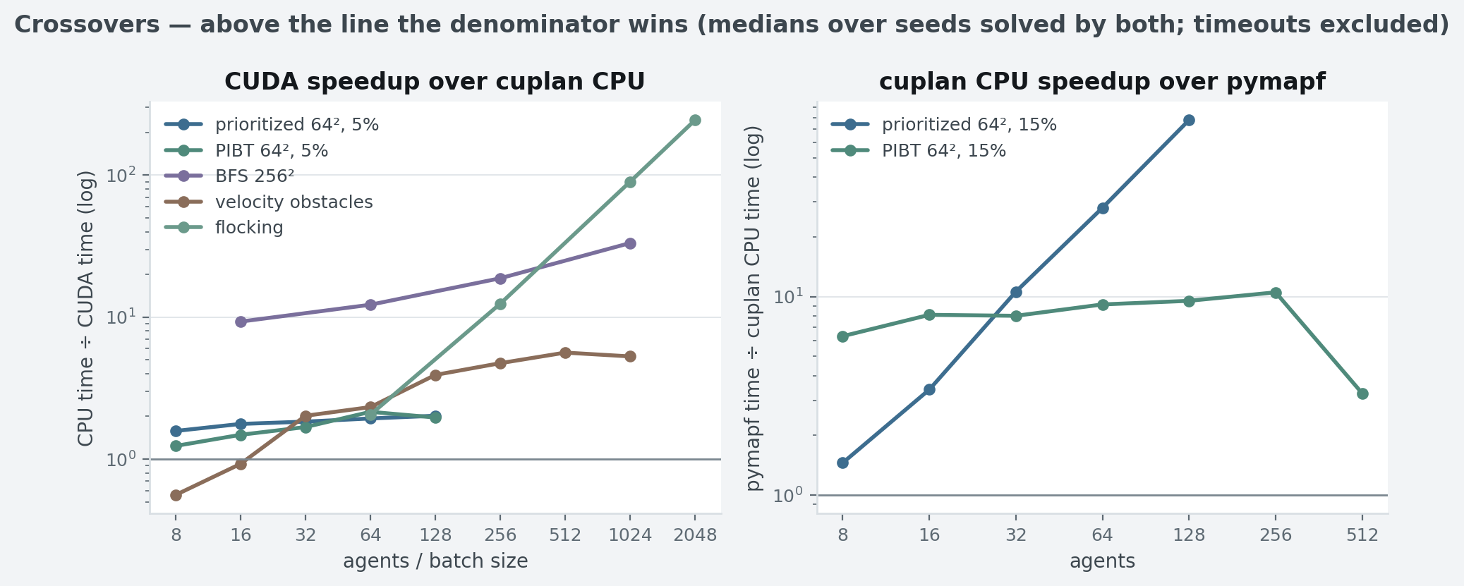
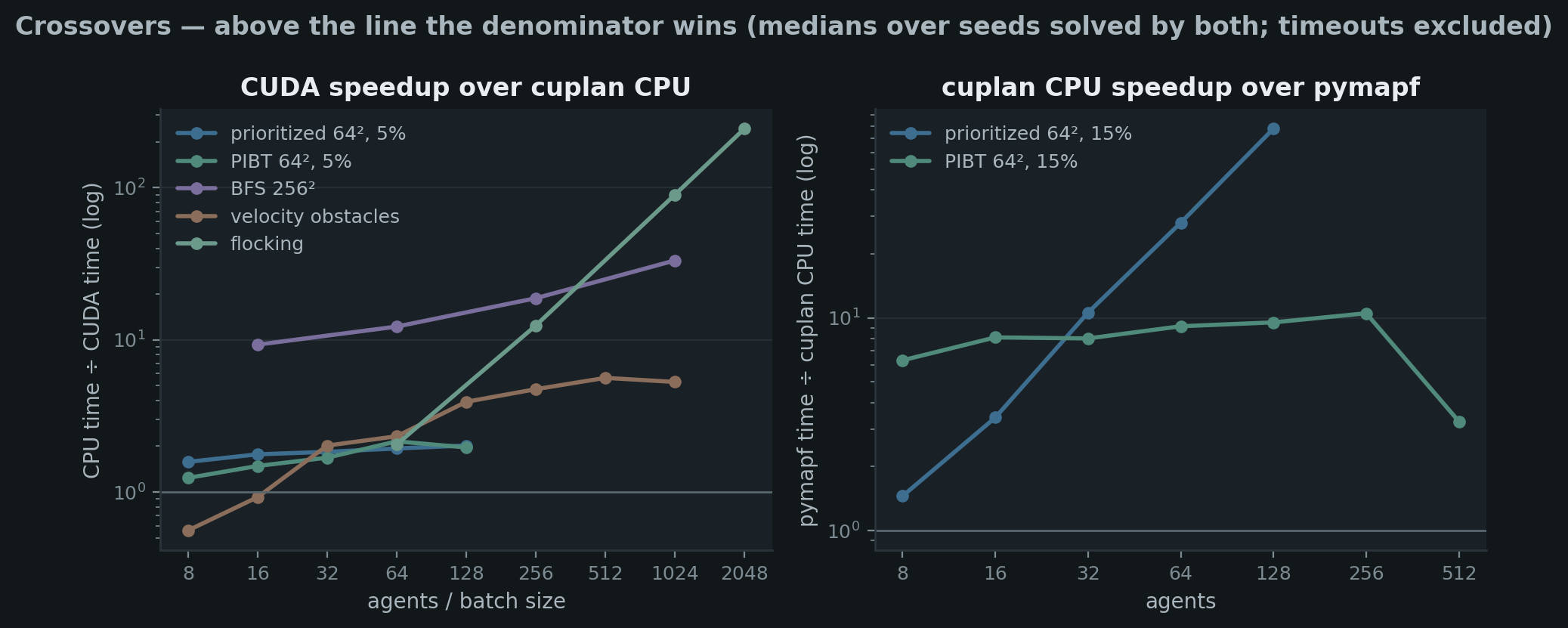
Median of per-seed runtime ratios on instances both solvers solved; timeouts excluded, which understates pymapf's deficit wherever it hit the 60 s cap. Left panel: cuplan CPU ÷ cuplan CUDA — above 1, the device wins. MAPF series are the 64² grid at 5% density, the only density where the CUDA arm survives. Right panel: pymapf ÷ cuplan CPU, MAPF series on the 64² grid at 15% density, where both those arms are complete. Both axes are log; the x-axis is agents for every family except BFS, where it is distance maps per batch.

family	CUDA beats CPU from	largest measured margin	conditions
Flocking	every swarm measured (≥64 agents)	245×	2048 agents, 200 steps
Batched BFS	every batch measured (≥16 maps)	33×	256² grid, 15%, 1024 maps
Velocity obstacles	~32 agents (0.9× at 16)	5.6×	512 agents, 80 steps
PIBT	64² grids and larger; a wash at 32²	2.2×	64² grid, 5%, 64 agents
Prioritized planning	every cell measured (≥8 agents)	2.0×	64² grid, 5%, 128 agents

Reading the left panel top to bottom is reading a spectrum of how GPU-shaped a workload is:

Flocking is the ideal case — one thread per agent, an O(n²) neighbour scan out of registers, 200 steps to amortize the launches, and no host work between them. It climbs steeply and only bends when the device saturates around 2048 agents.

Batched BFS starts high (9.4× at 16 maps on 256²) and rises slowly, because it is kernel-bound from the first bar — 97% of CUDA wall time is kernel at every batch size. Its wins come from amortizing a launch count that scales with the graph diameter, not with the batch.

Velocity obstacles is the only family that starts below the line: 0.56× at 8 agents. At that size the kernel is 60% of wall time and the fixed per-step costs — three small uploads, 80 times over — are the rest. It crosses between 16 and 32 agents and then plateaus around 5–6×, because each thread's scan over the other agents grows as the agent count does.

The MAPF families barely move, for two different reasons that both come down to Amdahl's law. In prioritized planning the phase breakdown puts 87–89% of CUDA wall time in the per-agent space-time wavefront, a loop that is sequential in the priority order: the GPU deleted the oracle and made each individual search faster, and the priority order owns the rest. In PIBT the device does even less — it builds the distance oracle and nothing else, because the inheritance chains are recursive and data-dependent and run on the host in both backends. Both sit between 1× and 2.2×, and neither trends upward with agents. Escaping that needs a solver that plans agents concurrently, which is a roadmap item, not a tuning problem.

The right panel is the algorithmic comparison, and it has a different shape per family. Prioritized planning's advantage over pymapf grows — 1.5× at 8 agents to 78× at 128 — because pymapf's per-agent cost rises with how full the reservation table already is while cuplan's dense lookup does not. PIBT's advantage is flat at 6–11× wherever more than one seed solved on both sides, because PIBT does a fixed amount of work per agent per step regardless of history. Same two libraries, same machine, two completely different curves; which one you get depends on the algorithm, not on the library.

Per-family pages

Page	What it settles
Prioritized planning	agents × grid × density scaling, success rates, quality vs pymapf
PIBT	why the pymapf ratio is flat, why the GPU needs a 64² grid
Batched BFS	the primitive alone; the family with no crossover
Velocity obstacles	the clearest CPU→GPU crossover in the library
Flocking	the largest speedup, and where it saturates
Phases and crossover	H2D / kernel / D2H / host splits — the why under all of the above
Methodology	machine, instance generation, timing protocol, what was cut

What is missing

This sweep is incomplete, and in one specific way. The MAPF stage runs last, and partway through it the CUDA driver entered a cudaErrorUnknown state that every subsequent context creation inherited. The sweep kept going and recorded 132 error rows rather than pretending the cells did not exist. In consequence:

• cuplan CUDA MAPF data exists for the whole 32² grid (all three densities, 8–128 agents) and for the 64² grid at 5% density only (8–128 agents, with the 128-agent cell resting on fewer than three seeds).
• cuplan CUDA MAPF data does not exist for 64² at 15% and 25%, for any of 128², or for 256² at all.
• The 256² grid was never reached for MAPF by any solver: the sweep's configured size axis is {32, 64, 128, 256} and the CSV stops at 128. The 128² grid itself only completed at 5% density.
• Everything else is complete. The BFS, velocity-obstacle, flocking and phase stages all ran to the end before the fault, on their full configured axes, and no figure on those pages is missing a cell.

What that costs the argument: the CUDA-versus-CPU MAPF ratios above are measured on sparse grids up to 64², so treat "~2× for prioritized planning" as characterised at that scale and unverified beyond it. The CPU-versus-pymapf comparison is unaffected — it is complete across all three grids and all three densities — and so is every primitive-family result. Re-running the missing cells is a matter of deleting the error rows and re-invoking the sweep, which resumes from the CSVs; the methodology page has the commands.