Benchmarks

Every number on this page was measured, and comes with its conditions.

The detailed study lives in Experiments

This page is the quick overview from the primary matrix. The full sweep — agents × grid × density scaling for every family, solution quality against pymapf on identical instances, success-rate heatmaps, CUDA phase breakdowns and the crossover analysis — is in the Experiments section, with raw CSVs committed alongside. Start at the summary for the headline table and the crossovers, or the methodology for the conditions and an accounting of the cells that sweep did not reach.

Machine — NVIDIA RTX A2000 Laptop GPU (4 GB, driver 560.35.03, CUDA 12.6) and its host CPU (x86_64); Python 3.10, CuPy 14.2 (cupy-cuda12x), NumPy under the CPU backend. Problems — random grids at 15% obstacle density, starts and goals drawn from one connected component, seeds {0, 1, 2}; identical seeded instances handed to every solver; medians over seeds. Timing — wall time for the full solve() call, host/device transfers included: the number a user sees. Reproduce — python -m cuplan.benchmark --out results (primary matrix), plus --sizes 128 --agents 32 64 128 256 --no-pymapf --bfs-sizes 256 --bfs-batches 1024 --vo-agents 256 512 for the large-scale extension. Raw CSV, aggregated tables and charts are committed under benchmarks/results/.

Costs are a correctness check as much as a speed one: cuplan's CPU and CUDA backends return identical solutions (the backends move the same algorithm, not a different one), and pymapf's costs on the same instances differ only by tie-breaking.

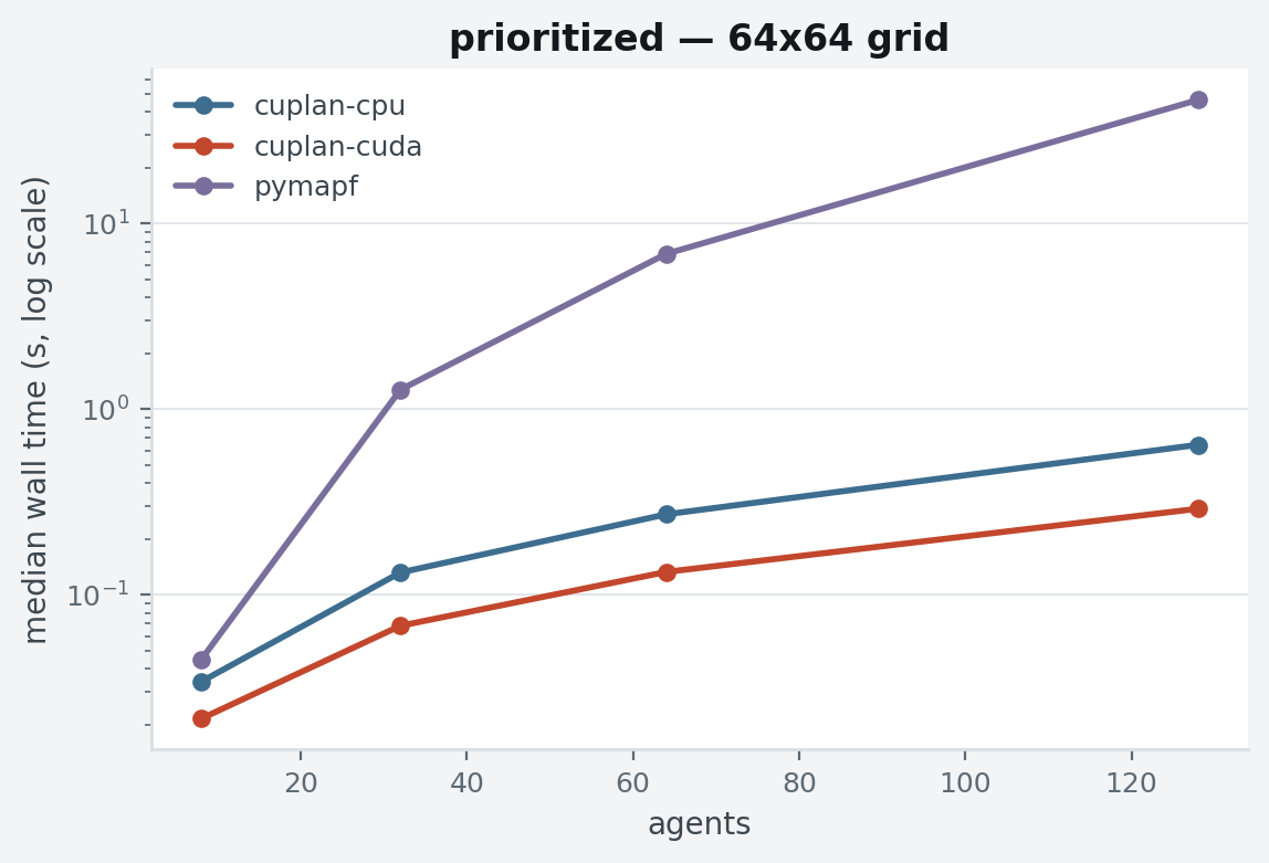
Prioritized planning

grid	agents	pymapf	cuplan CPU	cuplan CUDA
32×32	32	0.298 s	0.064 s	0.045 s
32×32	128	15.75 s	0.249 s	0.175 s
64×64	64	6.870 s	0.272 s	0.133 s
64×64	128	46.34 s	0.643 s	0.291 s

Two things are being measured at once: the wavefront formulation (dense reservation lookups instead of set membership — most of the CPU-vs-pymapf gap) and the GPU itself (the remaining ~2× on top). All three solvers fail the same 32×32 / 128-agent seed — prioritized planning is incomplete, and cramming 128 agents into 870 free cells is where it shows.

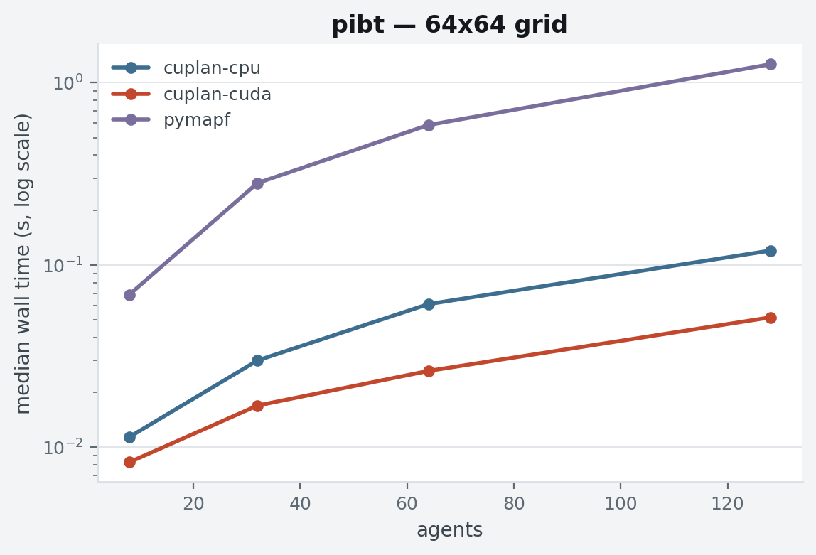
PIBT

grid	agents	pymapf	cuplan CPU	cuplan CUDA
32×32	64	0.154 s	0.020 s	0.014 s
64×64	64	0.586 s	0.061 s	0.026 s
64×64	128	1.263 s	0.120 s	0.052 s

The GPU accelerates the distance oracle and nothing else: one batched BFS instead of a Dijkstra per agent, built once before the first timestep. The per-step candidate ranking and the inheritance chains are host NumPy in both backends, so the gap narrows as the step loop dominates the oracle — visible in dense 32×32 instances.

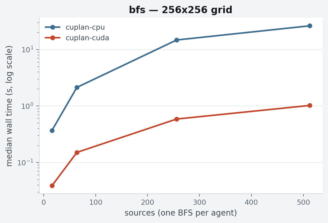
Batched BFS distance maps

grid	maps	cuplan CPU	cuplan CUDA	speedup
64×64	512	0.333 s	0.023 s	14×
128×128	512	2.988 s	0.157 s	19×
256×256	256	14.80 s	0.589 s	25×
256×256	512	26.37 s	1.025 s	26×

The primitive underneath everything else, measured alone. Kernel launches scale with graph diameter, not batch size, so the speedup grows with both grid and batch. pymapf has no batched equivalent; its per-goal Dijkstra cost is inside the solver timings above.

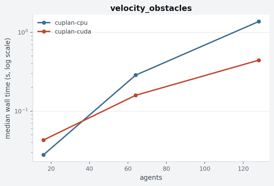
Velocity obstacles

agents	cuplan CPU	cuplan CUDA
16	0.028 s	0.043 s
64	0.286 s	0.159 s
128	1.371 s	0.443 s

80 timesteps, agents on a circle with antipodal goals. The CPU wins at 16 agents — kernel-launch overhead dominates an (agents × samples) grid that small — and the crossover sits between 16 and 64 agents. pymapf is absent from this family on purpose: its simulator updates agents sequentially within a timestep (earlier agents do not see later ones), so a wall-clock comparison would time two different problems; see the semantics note.

Large-scale extension (cuplan only)

128×128 grids and batch sizes past the primary matrix, same protocol, pymapf omitted (its prioritized planner needs minutes per instance at this scale — extrapolate from the 64×64 table). All instances solved by both backends, identical costs.

workload	cuplan CPU	cuplan CUDA	speedup
Prioritized, 128×128, 256 agents	4.53 s	1.14 s	4.0×
PIBT, 128×128, 256 agents	1.17 s	0.22 s	5.2×
Batched BFS, 1024 maps on 256×256	54.25 s	1.86 s	29×
Velocity obstacles, 512 agents × 80 steps	23.23 s	5.56 s	4.2×

The trend from the primary matrix continues: the CUDA margin grows with scale, and a 4 GB laptop GPU sustains 256-agent prioritized planning at interactive rates. Raw data: benchmarks/results/large/.

Reading the numbers

• The GPU pays off through batch size: many agents, many queries, many samples. Below a few dozen agents, backend="cpu" is the right choice — backend="auto" exists because the crossover is workload-dependent, not because CUDA always wins.
• Success rates below 100% are the honest face of incomplete solvers, not measurement noise; the same instances fail across libraries.
• A laptop-class 4 GB GPU produced all of the above. Larger devices raise the ceiling (batch sizes, grid sizes), not the shape of the curves.