Prioritized planning

Prioritized planning (Erdmann & Lozano-Pérez 1987) in the space-time A* form of Silver (2005): agents are planned one at a time in a fixed priority order, each one routed through a reservation table holding every path already committed. It is fast and incomplete — a low-priority agent can be boxed in by a choice made earlier, and no amount of compute recovers from it.

Conditions for the whole page: random grids from random_scenario, starts and goals in one connected component, seeds {0, 1, 2}, the same instance object handed to all three solvers, medians over seeds with min–max bands, wall time including host/device transfers, caps of 60 s (pymapf) and 300 s (cuplan). Full protocol on the methodology page, which also records why the CUDA arm stops where it does.

Scaling with agents

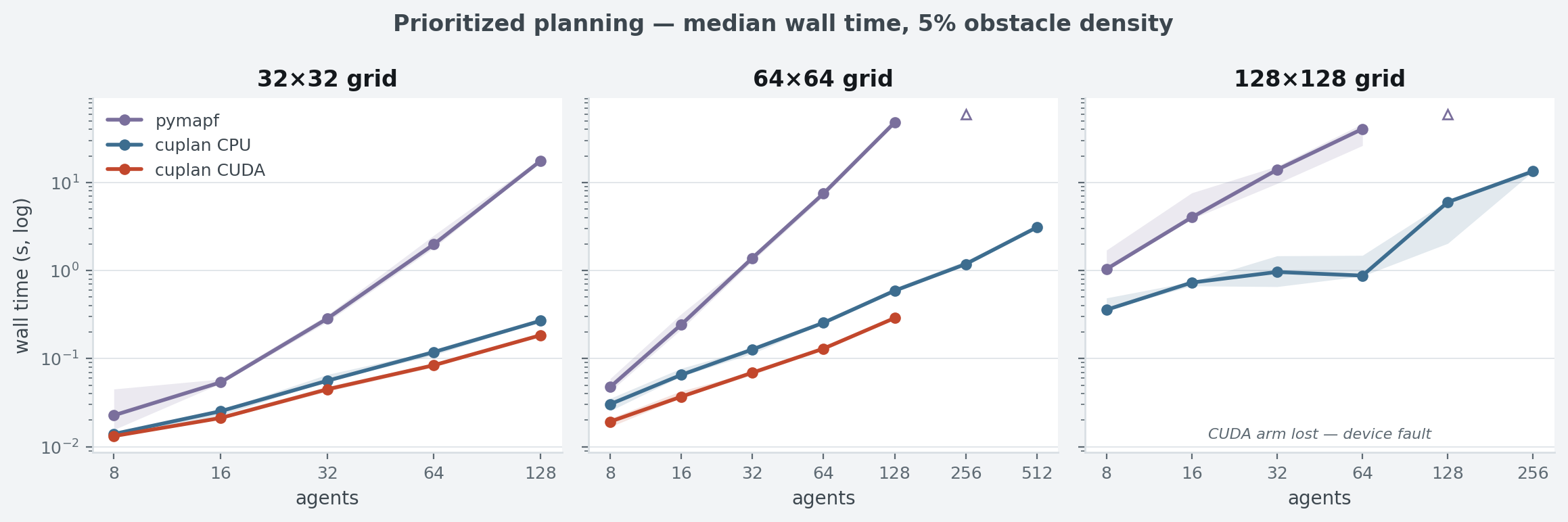
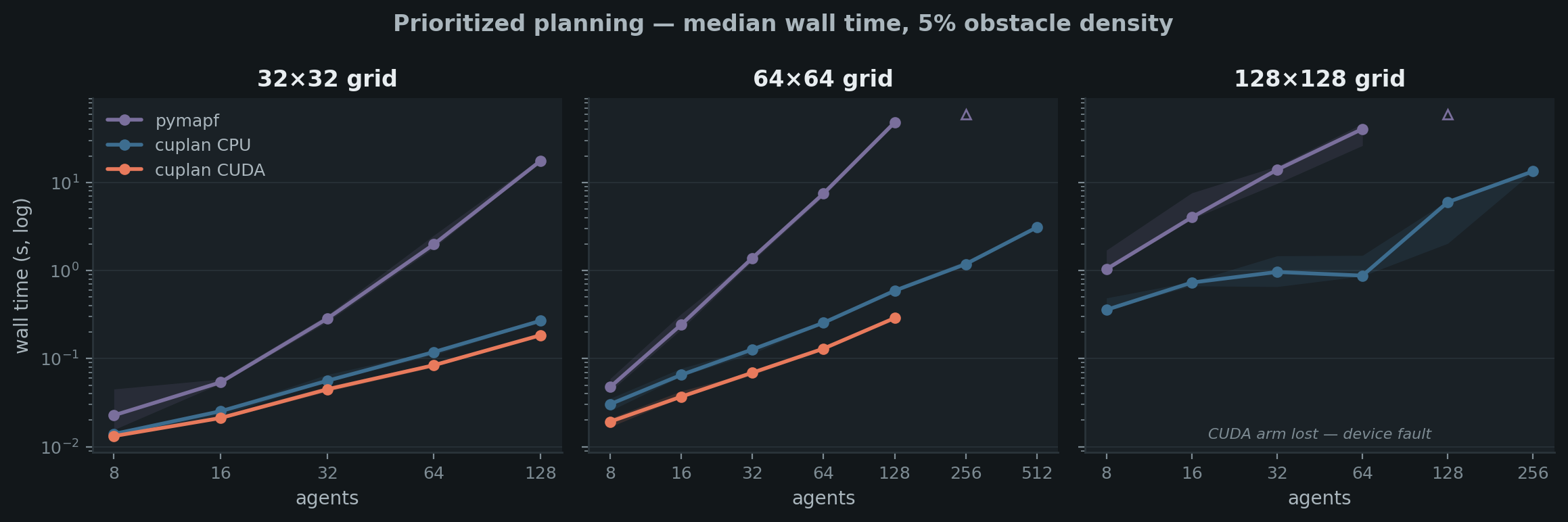
Median wall time, log–log, at 5% obstacle density — the one density reached on all three grids before the sweep was interrupted. Grids 32², 64², 128²; agents 8–512; seeds {0, 1, 2}; bands are min–max over seeds that solved. Hollow triangles are pymapf runs stopped at the 60 s cap, plotted at the cap and never extrapolated. The 128² panel has no CUDA line: those cells are on disk as device errors, not as measurements.

The three lines separate for two different reasons, and it is worth keeping them apart.

pymapf → cuplan CPU is an algorithmic gap, and it widens. On the 64² grid the ratio runs 1.6× at 8 agents, 10.9× at 32, 28.1× at 64, 78.5× at 128 — the curve is bending away, not offset. Both libraries run the same algorithm, so the divergence is in the data structures: pymapf builds one Dijkstra table per agent and tests reservations against a growing set, so its per-agent cost rises with the number of agents already placed; cuplan builds all the distance tables in one batched BFS and tests reservations by indexing a dense (horizon, H, W) array, which is O(1) no matter how full the table is. Superlinear against near-linear, on a log axis, is a bend.

cuplan CPU → cuplan CUDA is a hardware gap, and it is modest. 1.6×–2.0× across the 64² row; 1.1×–1.5× on 32². It does not widen much because most of the work cannot be parallelized: the phase breakdown puts 87–89% of CUDA wall time in the per-agent space-time wavefront, whose depth is one agent's path length. The GPU deleted the oracle (3.5% of the budget at 64², 64 agents) and made each individual search faster, and what remains is Amdahl's law over the priority order. A solver that plans agents concurrently — LaCAM-style — is the only thing that moves this number, and it is on the roadmap, not in the box.

The margin grows with the grid, not with the agent count. 32² → 64² takes CUDA from ~1.3× to ~1.9× at the same 32 agents, because a wavefront on a 64² grid has four times the cells to expand in parallel per launch while the number of launches (the path length) only doubles. The device is fed by grid area; agents mostly buy more sequential iterations.

Selected medians, 64×64 grid, 5% density

agents	pymapf	cuplan CPU	cuplan CUDA	CUDA vs CPU	pymapf vs CPU
8	0.048 s	0.030 s	0.019 s	1.6×	1.6×
16	0.244 s	0.065 s	0.037 s	1.8×	3.3×
32	1.39 s	0.127 s	0.069 s	1.8×	10.9×
64	7.49 s	0.255 s	0.130 s	1.9×	28.1×
128	47.95 s	0.590 s	0.289 s ²	2.0×	78.5×
256	timeout at 60 s	1.19 s	— ¹	—	≥50×
512	not run ³	3.10 s ⁴	— ¹	—	—

Medians over 3 seeds unless noted. Ratios are medians of per-seed ratios on instances both solvers solved, so they are not exactly the ratio of the two median columns. ¹ CUDA rows lost to the device fault. ² 2 seeds — the third is the first row the fault touched. ³ pymapf skipped by timeout escalation after all 3 seeds timed out at 256 agents. ⁴ 2 of 3 seeds solved; the median is over those two.

The 60 s cap is doing real work in that table. At 256 agents on 64², every pymapf seed hit it while cuplan's CPU backend finished in 1.19 s — so the true ratio is at least 50×, and the honest form of the claim is a lower bound, not a number.

Density

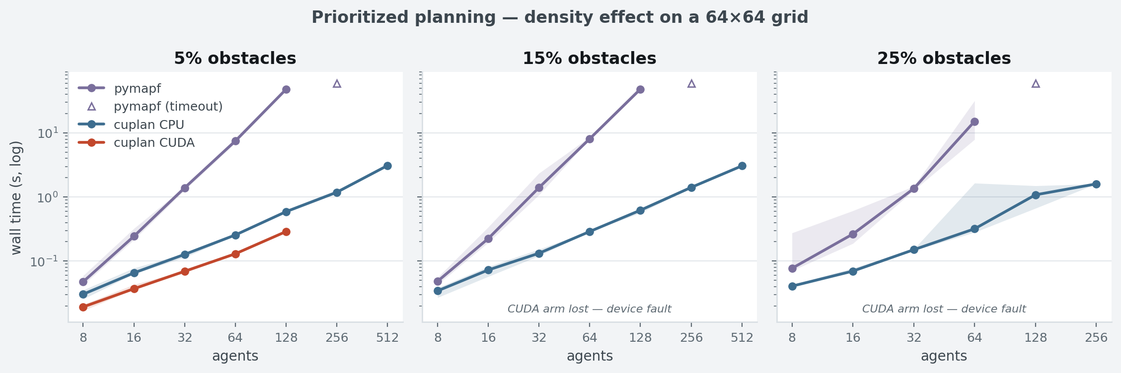
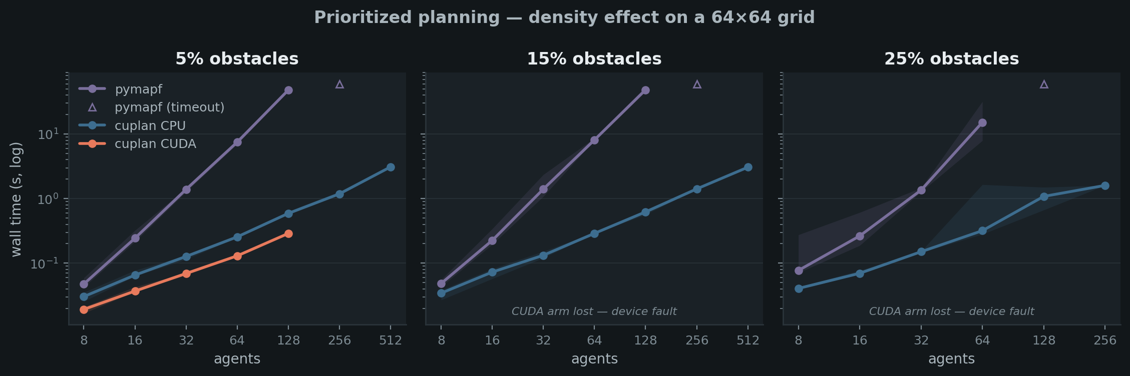
64×64 grid, obstacle density 5% / 15% / 25%, agents 8–512, seeds {0, 1, 2}, shared y-axis. The 15% and 25% panels carry no CUDA line: the device fault reached the sweep before those cells ran.

Density barely moves the runtime curves and moves the failure curve a lot. cuplan CPU at 64 agents costs 0.255 s at 5%, 0.289 s at 15%, 0.319 s at 25% — a 25% spread across a fivefold change in obstacle count, because the wavefront visits free cells and obstacles simply remove cells from the search. What density changes is how often a low-priority agent finds nothing left to reserve, which is the next figure and not this one.

Success rate

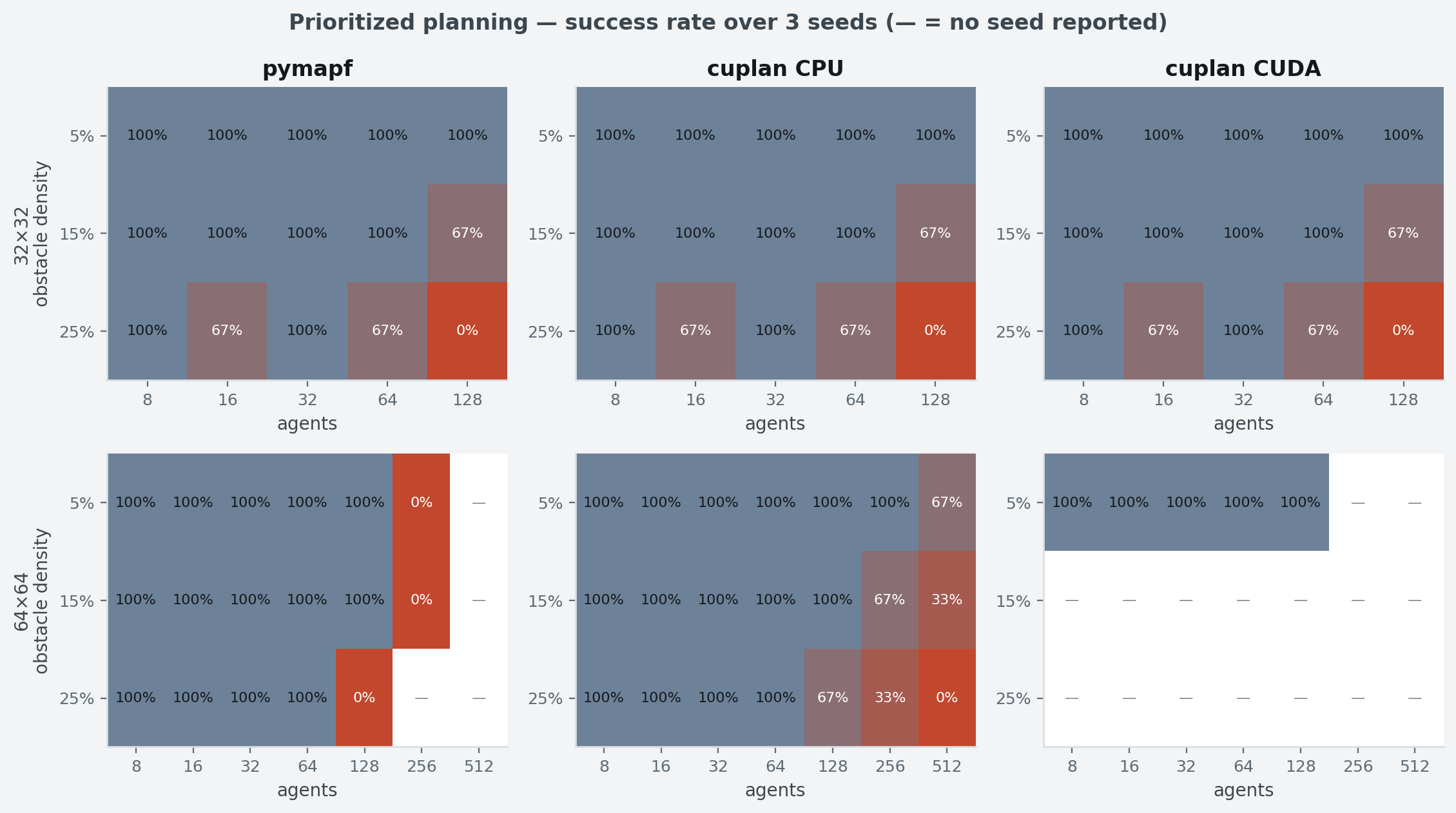
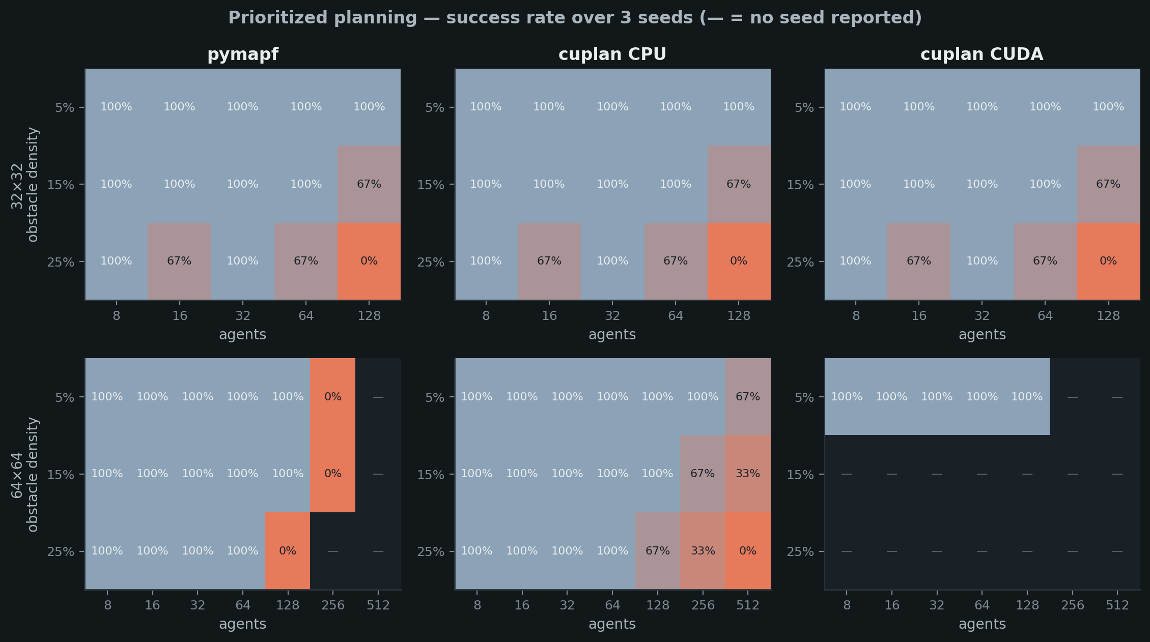
Fraction of seeds returning a plan that passes cuplan's independent validator. Rows are grids (32², 64²), columns are solvers, cells are agents × obstacle density over seeds {0, 1, 2}. A timeout counts as a failure, which is why pymapf shows 0% at 64²/256 agents while cuplan shows 100%. An em dash means no seed reported a result: for pymapf that is timeout escalation, for cuplan CUDA at 64² it is the device fault.

Two things this figure is for.

The failures agree across libraries. On the 32² grid every solver fails the same cells — 67% at (128 agents, 15%), 0% at (128, 25%), 67% at (16, 25%) — because incompleteness is a property of prioritized planning, not of an implementation. 128 agents in a 32² grid at 25% density is 256 endpoints in 768 free cells; a low-priority agent gets boxed in and the algorithm has no way back. Three independent solvers failing on exactly the same seeds is the strongest available evidence that they are running the same algorithm.

Where they disagree, it is the cap, not the solver. Every pymapf 0% cell on the 64² grid is a timeout, not a reported failure — read those as "did not finish in 60 s".

The single seed at (32², 16 agents, 25%) that all three fail is a useful reminder that success rate is not monotone in agent count: one bad start/goal draw beats a large easy instance. With 3 seeds a cell is resolved to ±33%, which is the resolution this sweep bought and no finer.

Solution quality

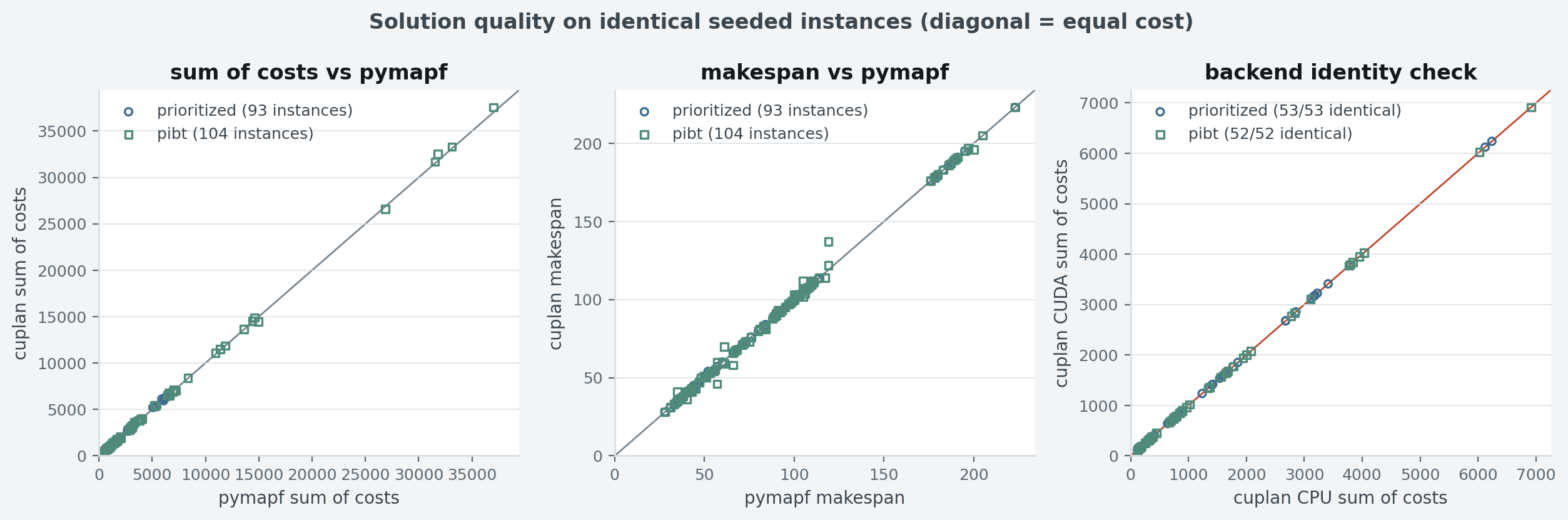
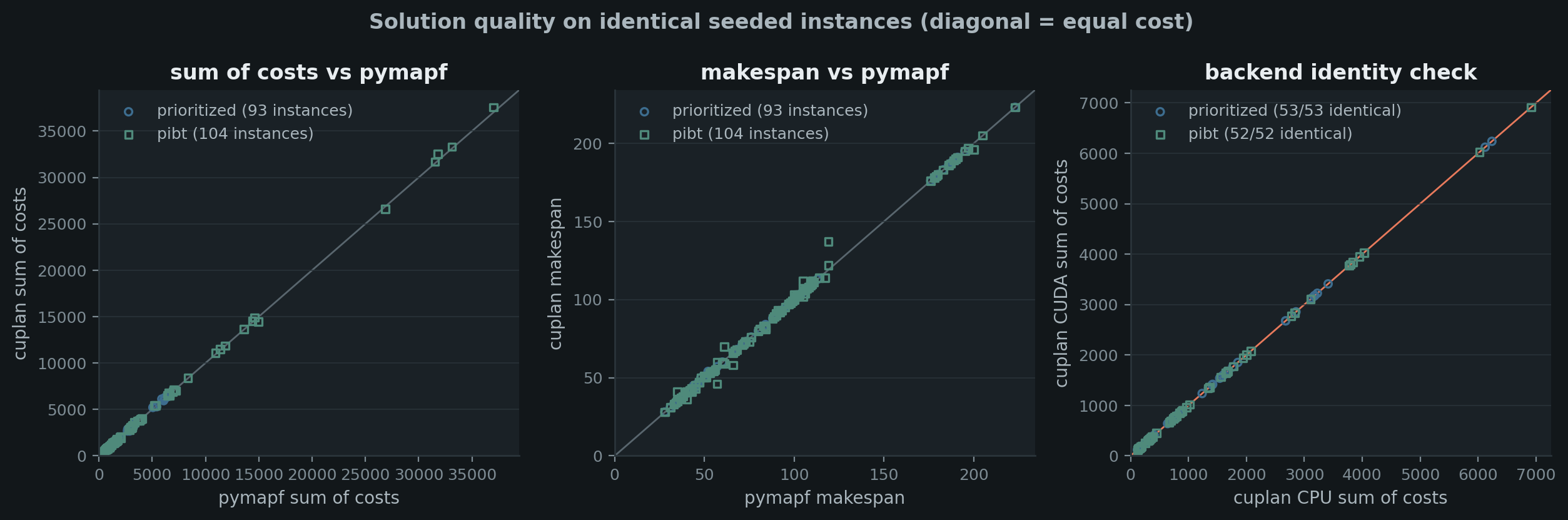
Every instance solved by both solvers, both MAPF families pooled: 93 prioritized and 104 PIBT instances for the pymapf panels, 53 + 52 for the backend check. Grids 32²–128², all three densities, seeds {0, 1, 2}. Diagonal = equal.

Speed claims are worthless without this figure. On the 93 shared prioritized instances the median cuplan/pymapf sum-of-costs ratio is exactly 1.0000, with a spread of 0.883× to 1.076×: cuplan is cheaper on 46% of them, dearer on 28%, and matches to the integer on 26%. The scatter has no drift off the diagonal in either direction, which is what tie-breaking noise looks like and not what a quality trade looks like. Neither implementation is optimal and neither claims to be; what this establishes is that the speedups above are not bought with worse plans.

The third panel is the stronger claim: on all 53 of 53 shared prioritized instances, cuplan's CPU and CUDA backends return the same sum of costs and the same makespan. Not close — equal. The backends move the same algorithm onto different hardware, and the test suite enforces it.

What to take away

• Below ~16 agents on a small grid, prioritized planning is already sub-50 ms on the CPU backend and the GPU is worth about 1.5×. Pass backend="cpu" and skip the device.
• The reason to reach for cuplan at all is the algorithmic gap, which is on the CPU backend too: 78× over pymapf at 64², 128 agents, 5% density, before any CUDA is involved.
• The reason to reach for the GPU specifically is a further ~2×, and it is capped there by the sequential priority loop. If you need more than that, the shape of the algorithm has to change.