Phases and crossover

The scaling pages show where CUDA wins; this page shows why — by timing what one CUDA call is made of. Conditions: same instance generators and seeds {0, 1, 2} as the scaling pages, device synchronization inserted at phase boundaries. Profiling itself costs a little, so these runs explain the headline totals but do not replace them.

Four phases, medians over seeds:

• H2D — copying inputs to the device and allocating outputs.
• kernel — the launched kernels, including each wave's 4-byte termination check for BFS.
• D2H — copying results back to NumPy.
• host — everything else: Python orchestration between launches.

The primitives

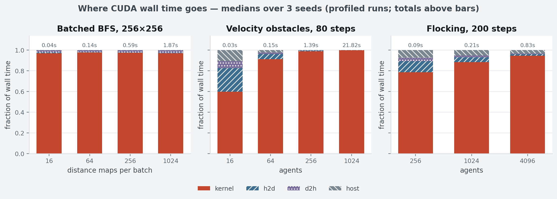
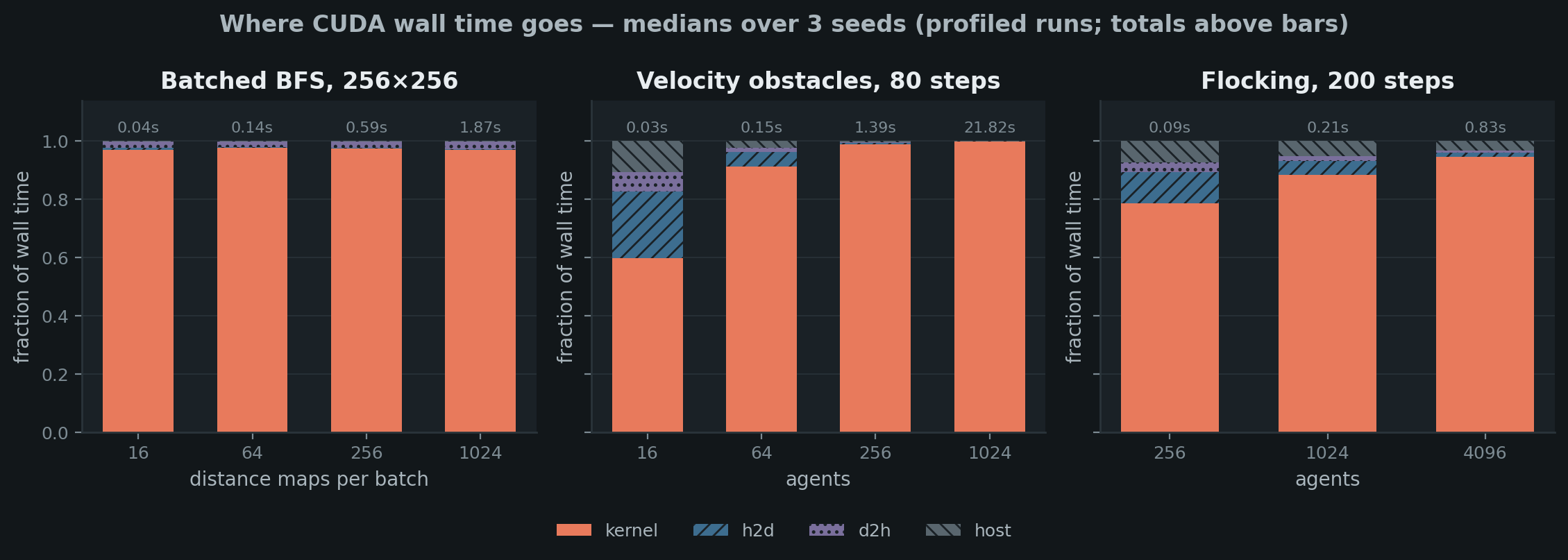
Stacked per-phase fractions; the label above each bar is the median total. BFS on a 256² grid at 15% density; velocity obstacles 80 steps; flocking 200 steps.

The three panels are three different answers to "is the GPU busy?":

• Batched BFS is kernel-bound from the first bar — 97–98% kernel at every batch size, transfers ~2–3%. That is why this family has no crossover: even 16 maps keep the device busier than the launch overhead costs. The uploaded grid is one byte per cell; the downloaded maps are the only real traffic and stay ~3%.
• Velocity obstacles is the crossover explained. At 16 agents the kernel is only 60% of wall time — 23% goes to H2D (three small uploads per step, 80 times) and 11% to host orchestration. Fixed per-step costs of ~0.16 ms swamp a 25 600-cone step (16² agent pairs × 100 velocity samples), and the CPU wins below ~32 agents. By 1024 agents the kernel is ~100% and the fixed costs have vanished into it.
• Flocking sits in between (78% kernel at 256 agents, 95% at 4096) but its per-step state is tiny — positions and velocities, not O(n²) — so the crossover still lands below the smallest measured swarm.

Prioritized planning, from the inside

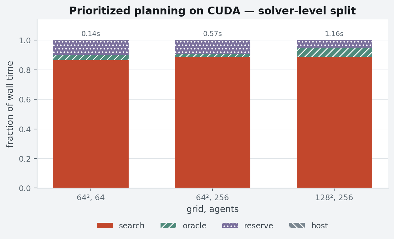
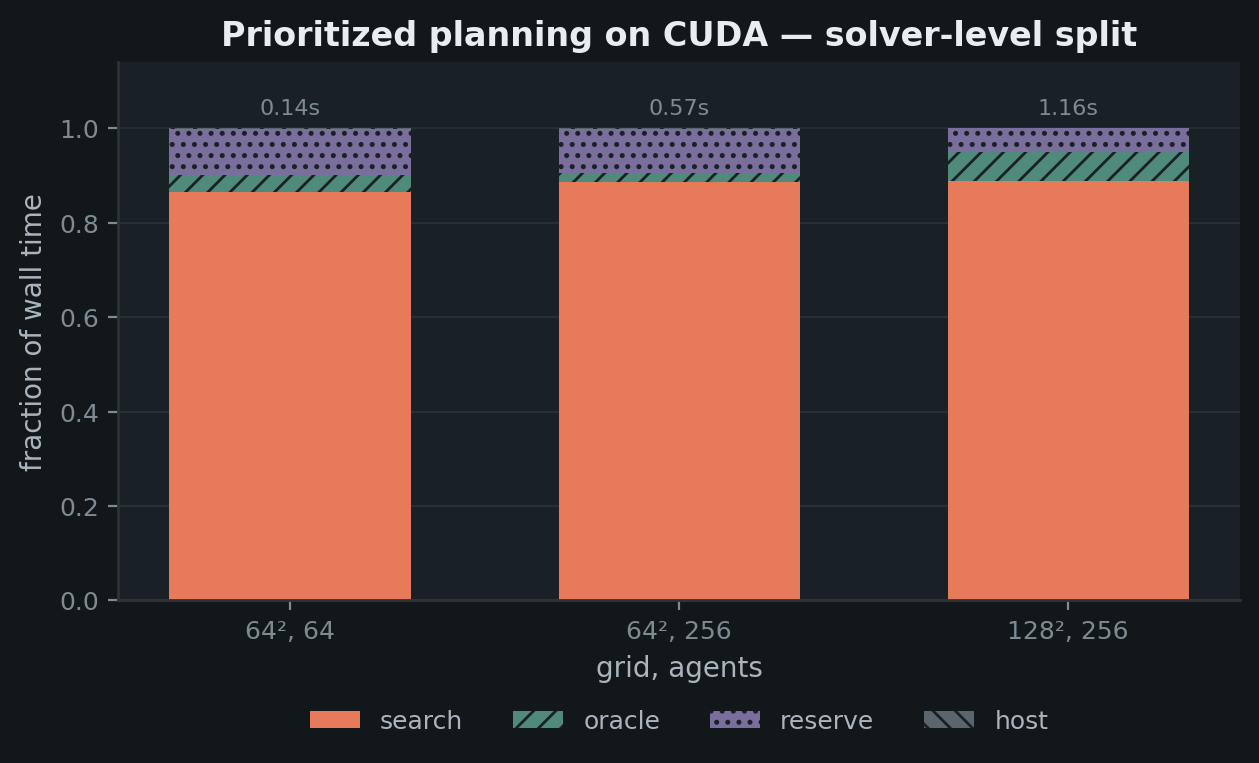
Solver-level split (this family's phases are algorithmic, not transfer-shaped): oracle = batched BFS heuristic tables, search = space-time wavefronts, reserve = reservation-table updates. 15% density, seeds {0, 1, 2}.

grid, agents	oracle	search	reserve	total
64², 64	3%	87%	10%	0.14 s
64², 256	2%	89%	9%	0.57 s
128², 256	6%	89%	5%	1.16 s

The oracle — the thing pymapf spends most of its time on, one Dijkstra per agent — is 2–6% of cuplan's budget, because it is one batched BFS. What remains is the sequential priority loop itself: ~90% of the time is the per-agent space-time wavefront, whose depth is the agent's path length and cannot be batched across agents without changing the algorithm. That is the honest ceiling of this design: the GPU removed the oracle and accelerated each search, and what is left is Amdahl's law over the priority order (LaCAM-style solvers attack exactly this — see the roadmap).

Throughput and saturation

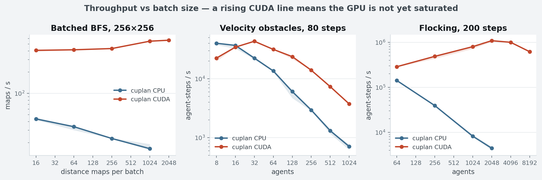
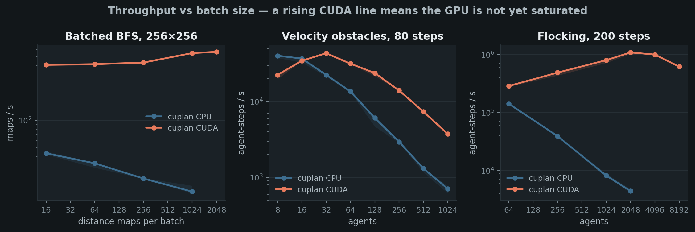
Median throughput (log–log): distance maps/s on a 256² grid, agent-steps/s for velocity obstacles (80 steps) and flocking (200 steps). Bands are min–max over seeds {0, 1, 2}.

A rising CUDA line means the device is not yet full: more work per launch is still free. BFS climbs through the whole measured range (407 → 566 maps/s on 256²; 25 800 maps/s on 64² grids). Flocking peaks at ~1.09 M agent-steps/s at 2048 agents, then eases down as each thread's O(n) neighbour scan grows. Velocity obstacles peaks much earlier (~43 000 agent-steps/s at 32 agents) because its per-step work grows O(n²) while its threads grow O(n) — the same shape, reached sooner. The falling CPU lines are the mirror image: O(n²) temporaries falling out of cache.

Crossover summary

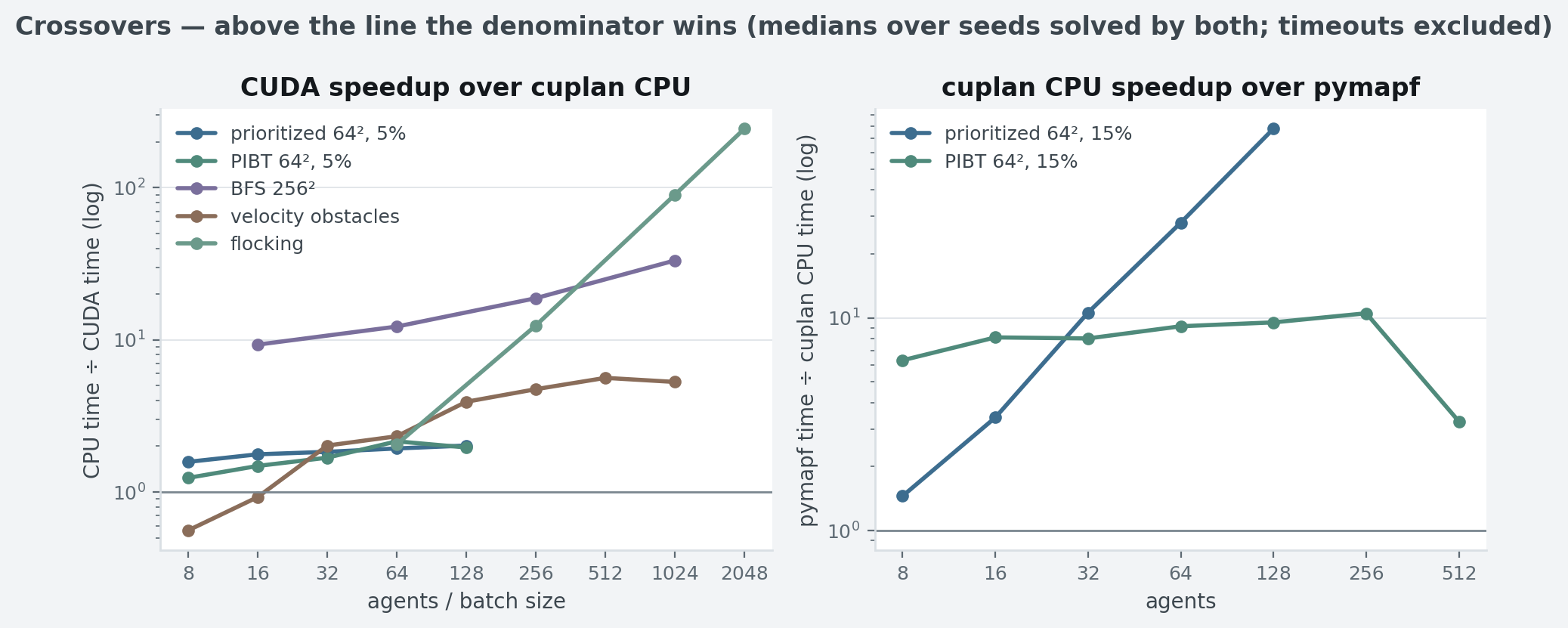
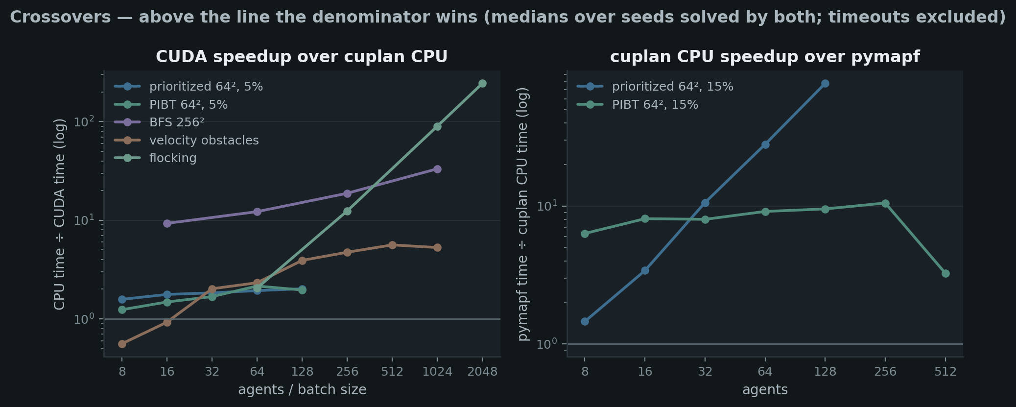
Median per-seed runtime ratios; solved seeds only, timeouts excluded (which understates pymapf's deficit above the 60 s cap). Left panel MAPF series are the 64² grid at 5% density — the only density whose CUDA arm survived the device fault. Right panel MAPF series are the 64² grid at 15% density, where both the cuplan CPU and pymapf arms are complete. See what is missing.

family	CUDA beats CPU from	largest measured margin
Flocking	every swarm measured (≥64 agents)	245× (2048 agents)
Batched BFS	every batch measured (≥16 maps)	33× (256², 1024 maps)
Velocity obstacles	~32 agents (0.9× at 16)	5.6× (512 agents)
PIBT	64² grids and larger; a wash at 32²	2.2× (64², 5%, 64 agents)
Prioritized	every cell measured (≥8 agents)	2.0× (64², 5%, 128 agents)

Note that the two MAPF rows say "grid", not "agents". Neither MAPF family's CUDA margin grows with the agent count — both stay between 1× and 2.2× across the whole measured range — because the priority loop above is sequential. What buys the GPU work in those families is grid area: more cells per wavefront launch. Prioritized planning runs ~1.3× at 32² and ~1.9× at 64² at the same 32 agents, and PIBT does not reliably win at 32² at all.

The rule the whole page argues for: the GPU pays through batch size. backend="auto" prefers CUDA when a device is present; on small grids and small swarms, pass backend="cpu" — the crossover is a property of the workload, not of the library. The summary page collects the crossovers and the headline numbers in one table.